- Home
- About Us
- Chapters
- Study Design and Organizational Structure
- Study Management
- Tenders, Bids, and Contracts
- Sample Design
- Questionnaire Design
- Instrument Technical Design
- Translation
- Adaptation
- Pretesting
- Interviewer Recruitment, Selection, and Training
- Data Collection
- Paradata and Other Auxiliary Data
- Data Harmonization
- Data Processing and Statistical Adjustment
- Data Dissemination
- Statistical Analysis
- Survey Quality
- Ethical Considerations
- Resources
- How to Cite
- Help

Statistical Analysis
Mengyao Hu, 2016
Appendices: A
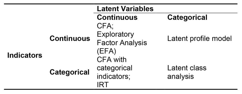
1.1 The classification of variable types is important, because it will help to determine which statistical procedure should be used. For example, when the dependent variable is continuous, a linear regression can be applied (see Guideline 2.2); when it is categorical (binary), a logistic model can be applied (see Guideline 3.2); when it is categorical (nominal or ordinal), multinomial, or ordinal, logistic regressions may be used (see Guideline 3.3). If, in latent variable models (see Guideline 6), the latent variable is continuous, confirmatory factor analysis (CFA) or item response theory (IRT) models can be used (see Guidelines 6.1 and 6.5). Figures 1 and 2 below list the choices of regression and latent variable measurement models as regard the variable types of the dependent and independent variables. Several commonly used variable types are listed as below:
-
- Nominal variables: variable values assigned to different groups. For example, respondent gender may be 'male' or 'female.'
- Ordinal variables: categorical variables with ordered categories. For example, 'agree,' 'neither agree nor disagree,' or 'disagree.'
- Continuous variables: variables which take on numerical values that measure something. “If a variable can take on any value between two specified values, it is called a continuous variable; otherwise, it is called a discrete variable” [zotpressInText item="{2265844:VU7LAK69}"]. Continuous variables are understood to have equal intervals between each adjacent pair of values in the distribution. Income is an example of a continuous variable.
- Discrete (ratio) variable: “a discrete variable can only take on a finite value, typically reflected as a whole number” [zotpressInText item="{2265844:2FC7WZ8U}"]. The variables have an absolute ‘0’ value. One example is the number of children a person has.
Figure 1: Variable types and choices of regression models.
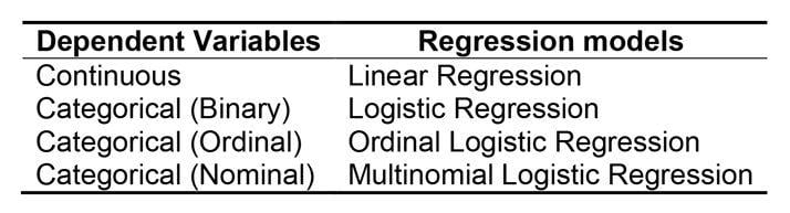
Figure 2: Variable types and choices of latent variable measurement models (see Guideline 6 for more detail).
1.2 Distribution of variables:
1.2.1 Graphical illustrations of distributions: it is commonly recommended to look at graphical summaries of both continuous and categorical distributions before fitting any models. Details of the graphical options listed below can be found in this online statistics book: Online Statistics Education: An Interactive Multimedia Course of Study.
-
-
- For categorical variables:
- Bar graphs
- Pie charts
- For continuous or discrete variables:
- Stem and Leaf Plots
- Histograms
- Box plots
- For any type of variable:
- Frequency distributions
- For categorical variables:
-
In 3MC data analysis, to get a direct visual comparison, researchers can plot distributions by country or racial group.
1.2.2 Numerical summaries of distributions: a distribution can be summarized with various descriptive statistics. The mean and median capture the center of a distribution (central tendency), while the variance describes the distribution spread or variability (see online book material).
-
-
- Mean: the average of a number of values. It is calculated by adding up the values and dividing by the number of values added.
- Median: the “…median is the number separating the higher half of a data sample, a population, or a probability distribution, from the lower half” [zotpressInText item="{2265844:8CIEV9P2}"]. For a highly skewed distribution, the median may be a more appropriate measure of central tendency than the mean. For example, the median is more widely used to characterize income, since potential outliers (e.g., those with very high incomes) have much more impact on the mean.
- Variance: a measure of the extent to which a set of numbers are 'spread out.'
- Precision: the reciprocal of the variance; most commonly seen in Bayesian analysis (see Guideline 9).
-
-
- Tests of the equality of two means (see online material)
- [zotpressInText item="{2265844:BGCZP7E8}" format="%a% (%d%)"]
- [zotpressInText item="{2265844:25BJAQUB}" format="%a% (%d%)"]
1.4 Potential uses in 3MC research:
-
- A good starting point for analysis is to look at the distributions of variables of interest and at graphical illustrations of the variables in each cultural group.
- One way of comparing survey estimates across various cultures is to directly compare mean estimates. A two-sample t-test can be used to evaluate the equality of two means (see Guideline 1.3). However, researchers need to be aware that the observed mean differences are not necessarily equal to the latent construct mean differences (see Guideline 6), and direct comparison using observed mean differences may lead to invalid results (see [zotpressInText item="{2265844:25BJAQUB}" format="%a% (%d%)"]). In addition, factors irrelevant to the question content, such as response style differences in different cultures, may influence the comparability across cultures. More advanced models (such as latent variable models) can be used to evaluate and control for these factors.
2. Simple and multiple linear regression models.
2.1 A bivariate relationship is the relationship between two variables. For example, one may be interested in knowing how height is associated with weight (i.e., whether those who are taller tend to weigh more). Basic information about bivariate relationships can be found here.
-
- Scatterplots: before running any models, a scatterplot is essential to explore the associations (negative or positive) between variables.
- Correlations between variables: Pearson's correlation is the most commonly used method of evaluating the relationship between two variables. Refer to this website for more information.
2.2 Linear regression models can allow researchers to predict one variable using other variable(s). The dependent variable in linear regression models is a continuous variable. Basic information about simple linear and multiple regression models can be found here.
-
- ANOVA table: in the output of regression model results, an analysis of variance (ANOVA) table is usually provided, consisting "of calculations that provide information about levels of variability within a regression model and form a basis for tests of significance" [zotpressInText item="{2265844:VCG42HHD}"].
- Dummy predictor variables: as described by [zotpressInText item="{2265844:C5T5K9R9}" format="%a% (%d%)"], a dummy variable or indicator variable is an artificial variable created to represent an attribute with two or more distinct categories or levels. If a categorical variable is added directly to the regression models without being specially specified, the software will treat it as continuous. However, the differences between the categories (e.g., category 2 minus category 1) do not have any actual meaning. Dummy variables are usually created in these situations to make sure that such categorical variables are correctly specified in the model. For example, in 3MC data analysis, to compare Country A to Country B on the level of the dependent variable, one can create a country dummy variable using one of the countries as a reference group and add it as an independent variable to the model. When multiple countries exist, one can use one of the countries as the reference category, and treat the variable as categorical in the model [zotpressInText item="{2265844:4SHZLPJQ}"].
- For information on dummy variables and how they are created and used, see [zotpressInText item="{2265844:C5T5K9R9}" format="%a% (%d%)"].
- For information on regression models with categorical predicators using SAS, see here.
- Interactions of predictor variables: sometimes a regression model is used to test whether the relationship between the dependent variable (DV) and one specific independent variable (IV) depends on another IV. To test this, an interaction term between the two IVs can be added to the model.
- Transformations of variables: when non-linearity is found for predictors, transformations may be considered to 'normalize' a variable which has a skewed distribution. For more detail, see [zotpressInText item="{2265844:QHFRARWG}" format="%a% (%d%)"].
- Lack of fit testing: various techniques are available to test for the lack of fit in regression models, including visual (e.g., plots) and numerical methods (e.g., [latex]R^2[/latex] and [latex]F[/latex]-tests).
- Model diagnostics: techniques are available to test the appropriateness of the model and whether the model assumptions hold.
- Resource 1
- Resource 2 (using R)
- Selecting reduced regression models (variable selection): techniques for determining the model which contains the most appropriate independent variables, giving the maximum [latex]R^2[/latex] value.
- Resource 1 (Including SAS code)
- [zotpressInText item="{2265844:X8GRKBLT}" format="%a% (%d%)"]
2.3 Suggested reading:
-
- Applied Statistical Analysis and Data Display: An Intermediate Course with Examples in S-PLUS, R, and SAS [zotpressInText item="{2265844:L9WA9P29}"]
- Statistical Methods, 8th ed [zotpressInText item="{2265844:D68X2GRG}"]
- The Little SAS Book, 4th ed [zotpressInText item="{2265844:4YHW698J}"]
2.4 Potential uses in 3MC research:
-
- As in linear regression models, a country variable/indicator can be added to the regression model as a covariate (e.g., [zotpressInText item="{2265844:4SHZLPJQ}" format="%a% (%d%)"]).
3.1 Analysis of two-way tables: categorical data are often displayed in a two-way table. Sometimes, one or both variables are continuous. If so, the continuous variable(s) can be categorized into groups. A two-way table can then be constructed using the new variables. Note that this approach may lead to a loss of information on the continuous variables. See also online marterial.
3.1.1 The Pearson chi-square test evaluates whether the row and column variables in a two-way table are associated.
3.1.2 Odds ratios (OR) and relative risks (RR) describe the proportions in contingency tables. See [zotpressInText item="{2265844:TMTIRUI5}" format="%a% (%d%)"] for a comprehensive introduction.
-
-
- Resource 1
- [zotpressInText item="{2265844:4HGGJSTK}" format="%a% (%d%)"]
-
3.1.3 Log-linear models are commonly used to model the cell counts of contingency tables such as two-way tables.
3.2 Logistic regression models: these can be used when the dependent variable is a binary categorical variable. The technique allows researchers to model or predict the probability that an individual will fall into one specific category, given other independent variables. Logistic regression is a type of generalized linear model where the logit function of selecting one category is expressed through a linear function of the predictors. Thus, as in other linear regression models, the predictors can include both continuous and categorical variables.
-
- [zotpressInText item="{2265844:EWYEBH24}" format="%a% (%d%)"] (link)
- Resource 2
3.3 Multinomial and ordinal logistic regressions: when the DV is a nominal variable, a multinomial logistic regression model can be used. If the DV is an ordinal variable, an ordinal logistic regression can be used.
3.4 Suggested reading:
-
- [zotpressInText item="{2265844:T75GI8TH}" format="%a% (%d%)"]
- [zotpressInText item="{2265844:IYNCVKER}" format="%a% (%d%)"]
- [zotpressInText item="{2265844:8ZNUHTUT}" format="%a% (%d%)"]
3.5 Potential uses in 3MC research:
-
- To evaluate responses to a categorical variable across two different cultures, one can construct a two-way table using the categorical variable and the country indicator as the rows and columns. A Pearson chi-square test can be used to evaluate whether the variable differs by cultures.
- As in logistic regression models, a country variable/indicator can be added to the logistic regression model as a covariate.
4.1 Suggested reading:
-
- [zotpressInText item="{2265844:3PP9GE9H}" format="%a% (%d%)"]
- [zotpressInText item="{2265844:X4EB3DYH}" format="%a% (%d%)"]
- [zotpressInText item="{2265844:ZGS8RB7M}" format="%a% (%d%)"]
- [zotpressInText item="{2265844:RLN9LPQ6}" format="%a% (%d%)"]
4.2 Potential uses in 3MC research:
-
- Many 3MC studies have a multilevel data structure with respondents nested within countries. Recent research on multilevel cross-cultural research has emerged in last several decades. For more information, see [zotpressInText item="{2265844:A8ZT4JUJ}" format="%a% (%d%)" etal="yes"].
5.1 Modeling longitudinal/panel data: in panel surveys, respondents are interviewed at multiple points in time, producing 'panel' or 'longitudinal' data. The first step in analyzing longitudinal data is to look at the descriptive plots; then, select one of several possible methods of analysis. The traditional technique is the repeated measures analysis of variance (rmANOVA), although this has several limitations. More commonly used approaches include multilevel models and marginal models.
5.1.1 Descriptive plots: The 'spaghetti' plot “involves plotting a subject’s values for the repeated outcome measure (vertical axis) vs. time (horizontal axis) and connecting the dots chronologically” [zotpressInText item="{2265844:FWNMNXX9}"]. Plots can be created at both the individual data level and the mean level. For binary outcomes, proportions can be used to generate the plot for different population groups. In 3MC studies, the plots can be generated for different cultural or country groups.
5.1.2 Repeated measures analysis of variance (rmANOVA):
-
-
- For more information, see this online example on rmANOVA.
- The rmANOVA approach is not recommended due to the limitations as mentioned below:
- Subjects missing any data will not be included in the analysis.
- A limited number of covariance structures are allowed.
- Time-varying covariates are not allowed.
-
5.1.3 Multilevel models for longitudinal data: multilevel models account for between respondent variance by including random effects in the model, such as random slope and random intercept.
-
-
- Resource 1
- Resource 2
- [zotpressInText item="{2265844:6T789TWT}" format="%a% (%d%)"] (presentation slides available here)
-
5.1.4 Marginal modeling approaches: If the between-subject variation is not of interest, the marginal modeling approach, where only the correlated error terms are included in the model, can be used—no random effects are added to the model.
-
-
- [zotpressInText item="{2265844:8S8REPVM}" format="%a% (%d%)"]
-
5.2 Suggested reading:
-
- [zotpressInText item="{2265844:ZP9BKGY3}" format="%a% (%d%)"]
- [zotpressInText item="{2265844:PNMHC6Z5}" format="%a% (%d%)"]
- [zotpressInText item="{2265844:6T789TWT}" format="%a% (%d%)"]
- [zotpressInText item="{2265844:W792PT3V}" format="%a% (%d%)"]
- [zotpressInText item="{2265844:53WEKKKD}" format="%a% (%d%)"]
- [zotpressInText item="{2265844:9ZRF85W2}" format="%a% (%d%)"]
- [zotpressInText item="{2265844:3UMDHSXD}" format="%a% (%d%)"]
- [zotpressInText item="{2265844:24T9INLQ}" format="%a% (%d%)"]
5.3 Potential uses in 3MC research:
-
- A country variable/indicator can be added to the marginal models as a covariate, or it can be added in a multilevel model as a fixed effect.
Latent variable models include both observed variables (the data) and latent variables. A latent variable is unobserved, which represents hypothetical constructs or factors [zotpressInText item="{2265844:UKUK5EDL}"]. A latent variable can be measured by several observed variables. An example of latent variable provided by [zotpressInText item="{2265844:UKUK5EDL}" format="%a% (%d%)"] describes the construct of intelligence. As mentioned by [zotpressInText item="{2265844:UKUK5EDL}" format="%a% (%d%)"], “there is no single, definitive measure of intelligence. Instead, researchers use different types of observed variables, such as tasks of verbal reasoning or memory capacity, to assess various facets of intelligence.” Examples of such latent variables are usually measured in a measurement model which evaluates the relationship between latent variables and their indicators.
6.1 Exploratory factor analysis (EFA) and confirmatory factor analysis (CFA): these are two types of measurement models where latent variables are indicated by multiple observed variables. The difference between EFA and CFA is related to the existence of a hypothesis about the measurement model before doing the analysis. As mentioned by [zotpressInText item="{2265844:NMXTNHHI}" format="%a% (%d%)"], “CFA attempts to confirm hypotheses and uses path analysis diagrams to represent variables and factors, whereas EFA tries to uncover complex patterns by exploring the dataset and testing predictions.” As seen in Figure 3, since both the indicators and the latent variables are all continuous, both EFA and CFA are based on linear functions. Figure 3 shows the differences between EFA and CFA. Since EFA is purely data-driven and may be arbitrary in nature, it is suggested by some literature to always use CFA, which is theory-driven [zotpressInText item="{2265844:3QNRDA6T}"]. However, as mentioned by [zotpressInText item="{2265844:3QNRDA6T}" format="%a% (%d%)" etal="yes"], in selecting items, it is more appropriate to use EFA rather than CFA when the theory is not well established.
See [zotpressInText item="{2265844:NMXTNHHI}" format="%a% (%d%)"] for a comprehensive overview on EFA and [zotpressInText item="{2265844:QLFEDAHM}" format="%a% (%d%)"] for CFA. The code for conducting EFA and CFA are included in Appendix A.
Figure 3: Comparisons between EFA and CFA*.
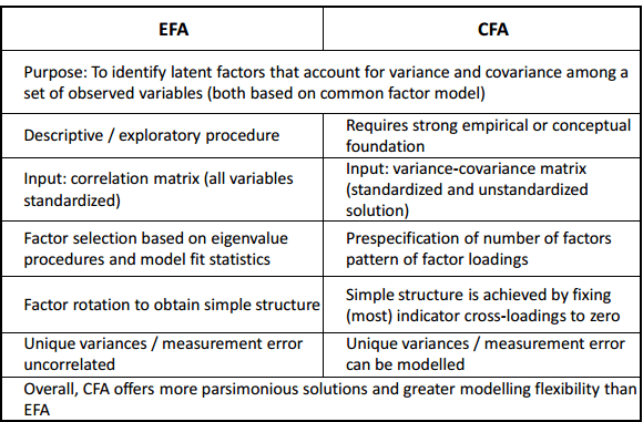
*Adapted from Exploratory and Confirmatory Factor Analysis presentation [zotpressInText item="{2265844:75DNFTE9}"].
Multigroup CFA (MCFA) is commonly used in 3MC research for measurement equivalence testing. The basic idea is to start with the same model, but allow the coefficients to differ by groups (assuming configural equivalence) and then start introducing constrains in the model coefficients—such as to make them equal across the groups. Then, the model fit of the previously run models can be compared. Among all the models, the parsimonious model with a good fit solution will be selected to evaluate the data. If the model reveals no violations of scalar equivalence, the country means can be compared directly. In a panel study, with data available at different time points, one can also evaluate measurement equivalence across cultures over time. See Guideline 6.2 below for more information on measurement equivalence testing. For more information on MCFA, see:
-
- Resource 1
- [zotpressInText item="{2265844:JEJTRWJQ}" format="%a% (%d%)"]
- [zotpressInText item="{2265844:QLFEDAHM}" format="%a% (%d%)"]
6.2 Measurement equivalence in 3MC research: as mentioned by [zotpressInText item="{2265844:J39XKRJQ}" format="%a% (%d%)"], “measurement equivalence implies that a same measurement instrument used in different cultures measures the same construct.” There are different levels of equivalence. Three of the most widely discussed levels are configural, metric, and scalar equivalence. These three levels are hierarchical, where the higher ones have higher requirements of equivalence and require the achievement of the lower ones [zotpressInText item="{2265844:J39XKRJQ}"].
Configural equivalence refers to similar construction of the latent variable. In other words, the same indicators are associated with the latent concepts in each culture. It does not require each culture to view the concept in the same way. For example, it allows the strength (i.e., loadings) to be different across cultures. Metric equivalence requires the same slope across cultures, which captures the associations between indicator and the latent variable. In other words, it implies “the equality of the measurement units or intervals of the scale on which the latent concept is measured across cultural groups” [zotpressInText item="{2265844:J39XKRJQ},{2265844:4SHTQ6YV}"]. Scalar equivalence implies that on the basis of equality of the measurement units, the scales of the latent variable also have the same origin across cultures [zotpressInText item="{2265844:J39XKRJQ}"]. Under this equivalence level, the model achieves full measurement equivalence, and researchers can compare the country scores directly.
In situations where full equivalence is difficult to achieve, researchers also evaluate the conditions under which different cultures achieve partial equivalence. An example of partial equivalence is when most of the indicators are equivalent across cultures, but only one has a different slope and threshold across cultures. One can then conclude that the different cultures achieve partial equivalence where they differ on one specific indicator. As mentioned by [zotpressInText item="{2265844:J39XKRJQ}" format="%a% (%d%)"], “partial equivalence enables a researcher to control for a limited number of violations of the equivalence requirements and to proceed with substantive analysis of cross-cultural data” [zotpressInText item="{2265844:J39XKRJQ},{2265844:4SHTQ6YV}"].
The aforementioned approaches to assessing measurement equivalence have been widely used in 3MC survey analysis. However, it has recently been criticized for being overly strict. As mentioned by [zotpressInText item="{2265844:VVR3R8GE}" format="%a% (%d%)"], it is difficult to achieve scalar equivalence, or even metric equivalence, in surveys with many countries or cultural groups. A Bayesian approximate equivalence testing approach has been recently proposed by [zotpressInText item="{2265844:VVR3R8GE}" format="%a% (%d%)" etal="yes"]. This approach allows for “small variations” in parameters across different cultural groups; thus, when approximate scalar measurement equivalence is reached, one can compare across cultures meaningfully, even though the traditional method may indicate scalar inequivalence [zotpressInText item="{2265844:VVR3R8GE}" etal="yes"]. [zotpressInText item="{2265844:36NZJE42}" format="%a% (%d%)"] point out that approximate measurement inequivalence or invariance are favorable for cases with large-scale data sets containing many groups or repeated measurements, small differences in intercepts and factor loadings, and multiple differences which are cancelled out both within and between groups. In contrast, approximate measurement invariance testing seems to lead to bias in latent mean estimates if large differences in intercepts or factor loadings or systematic differences between groups exist [zotpressInText item="{2265844:36NZJE42}" etal="yes"]. For introductions and references of Bayesian methods, see Guideline 9.
6.3 Latent class analysis (LCA): unlike the previously mentioned approach, such as CFA and SEM, where the latent variables are continuous, LCA treats the latent variables as categorical (nominal or ordinal) (see Figure 3). The categories of the latent variable in LCA are referred to as classes, which represent “a mixture of subpopulations where membership is not known but is inferred from the data” [zotpressInText item="{2265844:UKUK5EDL}"]. That is to say, LCA can classify respondents into different groups based on their attitudes or behaviors, such as classifying respondents by their drinking behavior. Respondents in the same group are similar to each other, regarding the behavior/attitudes, and they differ from those in other groups—i.e., heavy drinkers vs. non-drinkers. One can also add covariates to the model if those measures can influence the class membership. In a second step, the class membership from the model can then be used for followup analysis. For example, to better understand the differences between respondents, a logistic (or multinomial logistic, if more than two groups) regression model can be run in which selected covariates are used to predict class membership. Alternatively, to evaluate the influence of class membership on other variables, LCA can also be used in regression models as a covariate to predict other outcomes. For more information on LCA, please see:
-
- Resource 1
- [zotpressInText item="{2265844:JZ7XY7H7}" format="%a% (%d%)"]
As mentioned by [zotpressInText item="{2265844:UDB8XIPS}" format="%a% (%d%)"], when testing for measurement invariance with latent class analysis, “the model selection procedure usually starts by determining the required number of latent classes or discrete latent factors for each group. … If the number of classes is the same across groups, then the heterogeneous model is fitted to the data; followed by a series of nested, restricted models which are evaluated in terms of model fit.” That is to say, unlike multigroup CFA, the multigroup LCA will need to identify whether the number of classes are the same across groups before testing for models at different invariance levels. See [zotpressInText item="{2265844:UDB8XIPS}" format="%a% (%d%)" etal="yes"], [zotpressInText item="{2265844:6D5SNP33}" format="%a% (%d%)"], and [zotpressInText item="{2265844:U6I6P3AV}" format="%a% (%d%)"] for more information.
6.4 Structural equation modeling (SEM) is a multivariate analysis technique used in many disciplines which aims to test the causal relationship hypothesis between variables [zotpressInText item="{2265844:2IEBITQ8}"]. It usually includes two components: 1) the measurement model, which summarizes several observed variables using their latent construct (e.g., CFA as discussed in Guideline 6.1), and 2) the structural model, which describes the relationship between multiple constructs (e.g., relationships among both latent and observed variables).
6.4.1 Similar to previously discussed latent variable models, SEM can have both observed and latent variables, where observed variables are the data collected from respondents and latent variables represent unobserved construct and factors [zotpressInText item="{2265844:UKUK5EDL}"]. The observed variables which are used as measures of a construct are indicators of the latent variable. In other words, the latent variable is indicated by these observed variables. Besides observed and latent variables, SEM models also include error terms, similar to the error terms in a regression analysis. As mentioned by [zotpressInText item="{2265844:UKUK5EDL}" format="%a% (%d%)"], “a residual term represents variance unexplained by the factor that the corresponding indicator is supposed to measure. Part of this unexplained variance is due to random measurement error, or score unreliability.”
6.4.2 In SEM analysis, parameter estimation is done by comparing the model-based covariance matrix with the data-based covariance matrix. The goal of this approach is to evaluate whether the model with best fit is supported by the data—that is, whether the two covariance matrices are consistent with each other and whether the model can explain as much of the variance of the data.
6.4.3 Structural equation models can also estimate the means of latent variables. It also allows researchers to analyze between- and within-group mean differences [zotpressInText item="{2265844:UKUK5EDL}"]. In 3MC analysis, one can estimate the group mean differences on latent variables, such as those between two cultures.
6.4.4 Suggested reading:
-
-
- [zotpressInText item="{2265844:UKUK5EDL}" format="%a% (%d%)"]
- [zotpressInText item="{2265844:I2U93354}" format="%a% (%d%)"]
- [zotpressInText item="{2265844:4ZDKG57G}" format="%a% (%d%)"]
-
6.5 Item response theory (IRT) is commonly used for psychometric and educational testing, and is becoming more popular in 3MC analysis. It begins with the idea that when answering a specific question, the response provided by an individual depends on the ability/qualities of the individual and the qualities of the question item. As mentioned by [zotpressInText item="{2265844:FGCCCAIR}" format="%a% (%d%)"], “the mathematical foundation of IRT is a function that relates the probability of a person responding to an item in a specific manner to the standing of that person on the trait that the item is measuring. In other words, the function describes, in probabilistic terms, how a person with a higher standing on a trait (i.e., more of the trait) is likely to provide a response in a different response category to a person with a low standing on the trait.” Therefore, IRT allows researchers to model the probability of a specific response to a question item, given the item and the individual’s trait level.
The simplest IRT model is the Rasch model, also called the one-parameter IRT model, which assumes equal item discrimination (“the extent to which the item is able to distinguish between individuals on the latent construct” [zotpressInText item="{2265844:8Q3RETX7}"]. This model starts from the premise that the probability of giving a 'positive' answer to a yes/no question is “a logistic function of the distance between the item’s location, also referred to as item difficulty, and the person’s location on the construct being measured,” also known as the person’s latent trait level [zotpressInText item="{2265844:SQ3GKMAV}"]. There are other types of IRT models available as well, which can be categorized by the number of parameters and the question response option format (e.g., binary or multiple response options and whether ordinal or nominal). Table 1 below summarizes the different types of IRT models.
In a two-parameter (2PL) IRT model, an item discrimination parameter is also included in the model. The parameters are “analogous” to the factor loadings in CFA and EFA, since they all represent “the relationship between the latent trait and item responses” [zotpressInText item="{2265844:QLFEDAHM}"]. A three-parameter (3PL) IRT model also includes a 'guessing' parameter. It describes the situation wherein when a question can be answered by guessing, the probability of giving a correct answer is higher than zero even for those with low latent trait level.
For items with multiple response options (ordinal or nominal variables), polytomous IRT models can be used. See Table 1 for details. In this chapter, we will not discuss these models in detail. See suggested readings on IRT models for more information.
Table 1: Variable type and IRT model choices.
| Type of observed variable | Model |
| Binary | 1 parameter-logistic (1PL) model/Rasch model |
| 2PL model | |
| 3PL model | |
| Multiple response options (ordinal) | Graded response model/Thurstone/Samejima polytomous models |
| Partial credit model (PCM)/Graded PCM | |
| Multiple response options (nominal) | Rating scale model |
| Nominal response model/Bock’s model |
6.5.1 Suggested reading:
-
-
- [zotpressInText item="{2265844:FGCCCAIR}" format="%a% (%d%)"]
- [zotpressInText item="{2265844:TDHG5LC8}" format="%a% (%d%)"]
- [zotpressInText item="{2265844:MANKD64E}" format="%a% (%d%)"]
- [zotpressInText item="{2265844:UZYCS8HI}" format="%a% (%d%)"]
- [zotpressInText item="{2265844:LAYCJPYB}" format="%a% (%d%)"]
- [zotpressInText item="{2265844:SQ3GKMAV}" format="%a% (%d%)" etal="yes"]
-
6.6 Besides what is discussed above, other types of latent variable models are available. Some examples are listed below:
-
- The latent transition model is “a special kind of latent class factor model that represents the shift from one of two different states, such as from nonmastery to mastery of a skill, is a latent transition model” [zotpressInText item="{2265844:UKUK5EDL}"]. See these slides for more information.
- In latent profile models, the latent variable is categorical and the indicators are continuous. It is commonly used for cluster analysis. See [zotpressInText item="{2265844:9BZ3WVWC}" format="%a% (%d%)"] for more information.
- The mixed Rasch model is “a combination of the polytomous Rasch model with latent class analysis” [zotpressInText item="{2265844:5RT9J66F}"]. See [zotpressInText item="{2265844:5RT9J66F}" format="%a% (%d%)"] for more information.
- When we have data where the population of individuals are divided into different groups, such as in a 3MC context, multilevel structural equation modeling (MLSEM) can be used. This model decomposes individual data into within-group and between-group components, and can simultaneously estimate within- and between-group models [zotpressInText item="{2265844:AYW9CKRE}"]. For more information on MLSEM, see [zotpressInText item="{2265844:L8N9AE7E}" format="%a% (%d%)"].
6.7 Potential uses in 3MC research:
-
- As mentioned by [zotpressInText item="{2265844:MBWREQI3}" format="%a% (%d%)"], the observed mean does not equal the latent mean, where the observed mean is a function of item intercepts, factor loadings, and the latent mean. Similarly, “observed mean differences between two or more groups (e.g., cultures) do not necessarily indicate latent mean differences as unequal intercepts and/or factor loadings will also lead to observed differences” [zotpressInText item="{2265844:MBWREQI3}"]. To conduct more valid comparisons across different groups (e.g., cultures), measurement invariance testing is a widely used method which aims to evaluate whether the latent means of various groups are comparable. In other words, it evaluates whether the different groups differ in factor loadings and intercepts of the measures. See [zotpressInText item="{2265844:MBWREQI3}" format="%a% (%d%)"] for more information.
- Measurement invariance testing is usually conducted within the multigroup analysis (MGA) framework. The most commonly used method is multigroup confirmatory factor analysis (MGCFA) (e.g., [zotpressInText item="{2265844:MBWREQI3}" format-"%a% (%d%)"]). Other types of MGA include multigroup structural equation modeling (MGSEM) analysis (e.g., [zotpressInText item="{2265844:4TPY384A}" format="%a% (%d%)"]), multigroup latent class analysis (e.g., [zotpressInText item="{2265844:GCA2MPAS}" format="%a% (%d%)"]), multigroup IRT model (e.g., [zotpressInText item="{2265844:952BRNSR}" format="%a% (%d%)"]) and multigroup mixed Rasch model (e.g., [zotpressInText item="{2265844:5RT9J66F}" format="%a% (%d%)"]). See [zotpressInText item="{2265844:TDHG5LC8}" format="%a% (%d%)" etal="yes"] for more information.
- A recent paper by [zotpressInText item="{2265844:2JYYMWQF}" format="%a% (%d%)"] discusses misconceptions in measurement equivalence analysis. Using data from the World Values Survey, they show that “constructs can entirely lack convergence at the individual level and nevertheless exhibit powerful and important linkages at the aggregate level”.
- [zotpressInText item="{2265844:D4UXQGFK}" format="%a% (%d%)"] examine new approaches to measurement invariance evaluation in the context of international large-scale assessments (ILSAs), which aim to produce cross-national comparisons of student outcome measures (e.g., achievement, behaviors, and attitudes). [zotpressInText item="{2265844:D4UXQGFK}" format="%a% (%d%)" etal="yes"] begin by reviewing the extent to which exact measurement invariance could be confirmed; then, using data from the International Civic Citizenship Education Study 2009, they extend the CFA model to include partial invariance, indirect/covariate effects, and a Bayesian approach to evaluating the approximate invariance assumption. They find that the Bayesian approach, assuming a parsimonious variance procedure, can play a key role in evaluating measurement invariance across national samples used in ILSAs, and that the integration of a strong model with less stringent assumptions is sufficient for estimating comparable scores of the latent constructs and allows the reporting of a table charting mean comparisons across a large number of groups. Yet, a high degree of consistency between [zotpressInText item="{2265844:D4UXQGFK}" format="%a% (%d%)" etal="yes"]’s results and models assuming exact invariance indicates that previously published results are not invalidated in any substantial way.
7. Differential item functioning.
Differential item functioning (DIF) is a statistical concept developed to identify to what extent a question item might be measuring different properties for individuals of separate groups (i.e., ethnicity, culture, region, language, sex, etc.). It can be used as indicators for 'item bias' if the items function in a systematically different way across cultures. To detect DIF, different methods can be used, as listed below:
- Mantel-Haenszel (MH) statistic is regarded as a “reference” technique of detecting DIF due to its ease of use and the fact that it can be applied to small samples [zotpressInText item="{2265844:4RAC2ZL9}"]. The disadvantage of MH statistic is that it does not allow for statistical significance testing.
- Logistic regression can be used as an alternative method to detect DIF. For more information, see [zotpressInText item="{2265844:FR7GGGP4}" format="%a% (%d%)"].
- DIF can be detected using an IRT framework. Item characteristic curves (ICCs) of the same item but from different groups can be compared to evaluate whether there is DIF. For more information, see [zotpressInText item="{2265844:BAHY24WK}" format="%a% (%d%)"] and [zotpressInText item="{2265844:TDLU6LGL}" format="%a% (%d%)"].
Machine learning is “a general term for a diverse number of classification and prediction algorithms” [zotpressInText item="{2265844:QWJG89QV}"] which have applications in many different fields. Unlike statistical modeling approaches, machine learning evaluates the relationships between outcome variables and predictors using a “learning algorithm without an a priori model” [zotpressInText item="{2265844:QWJG89QV}" etal="yes"]. Below, we introduce several machine learning methods.
8.1 The classification tree is a data-driven method which allows researchers to evaluate the complex interaction between variables when there are many predictor variables present. In binary trees, the nodes of the tree are divided into two branches. To reasonably construct and prune a given tree, deviance measure is used to choose the splits. In R, the 'rpart' package is used for classification tree analysis (see Appendix A for more information). The classification tree result can be evaluated through apparent error rate and true error rate. The former is the error rate when the tree is applied to a training data set, and the latter is when it is applied to a new data set or to test data. In evaluating the true error rate, researchers usually divide the data into two parts—training data and test data—and validate the tree based on the test data set.
8.2 Random forest is an algorithm for classification which uses an “ensemble” of classification trees [zotpressInText item="{2265844:LVGZHQE7}"]. Through averaging over a large ensemble of “low-bias, high-variance but low correlation trees,” the algorithm yields an ensemble that can achieve both “low bias and low variance” [zotpressInText item="{2265844:LVGZHQE7}"].
8.3 Suggested reading:
-
- Resource 1
- Resource 2
- [zotpressInText item="{2265844:INXZ9N9Z}" format="%a% (%d%)"]
- [zotpressInText item="{2265844:NGK56WEJ}" format="%a% (%d%)"]
- [zotpressInText item="{2265844:A3U9G5UW}" format="%a% (%d%)"]
- [zotpressInText item="{2265844:BHC64GYX}" format="%a% (%d%)"]
8.4 Potential uses in 3MC research:
-
- Classification tree analysis in cross-cultural research allows researchers to evaluate 1) the important factors for each culture and 2) how the factor interactions differ across cultures. One study used classification tree to evaluate college student alcohol consumptions across American and Greek students, and found that “student attitudes toward drinking were important in the classification of American and Greek drinkers” [zotpressInText item="{2265844:QEXA7DK9}"].
9. Incorporate complex survey data features.
It is usually difficult to draw a simple random sample from the population due to cost and practical considerations such as no comprehensive sampling frame being available. As discussed in Sample Design, complex samples, such as surveys involving stratified/cluster sample design, are commonly used in surveys. In a simple random sample, one can assume that observations are independent from one another. However, in a complex sample design such as multi-stage samples of schools, classes, and students, students from one classroom are likely to be more correlated than those from another classroom. Therefore, as described in Sample Design, in the analysis phase, we need to compensate for complex survey designs with features including, but not limited to, unequal likelihoods of selection, differences in response rates across key subgroups, and deviations from distributions on critical variables found in the target population from external sources (such as a national census), most commonly through the development of survey weights for statistical adjustment. If complex sample designs are implemented in data collection but the analysis assumes simple random sampling, the variances of the survey estimates can be underestimated, and the confidence interval and test statistics are likely to be biased [zotpressInText item="{2265844:V657YFY4}"].
In a recent meta-analysis of 150 sampled research papers analyzing several surveys with complex sampling designs, it was found that analytic errors caused by ignorance or incorrect use of the complex sample design features were frequent. Such analytic errors define an important component of the larger total survey error framework, produce misleading descriptions of populations, and ultimately yield misleading inferences [zotpressInText item="{2265844:9JQS6IRI}"]. It is thus of critical importance to incorporate the complex survey design features in statistical analysis.
For many of the aforementioned statistical models, various statistical software programs, such as the 'svy' statement in Stata and SURVEY procedures in SAS, have enabled the analysis of complex survey data features. See Appendix A for more information.
-
- [zotpressInText item="{2265844:V657YFY4}" format="%a% (%d%)" etal="yes"]
- [zotpressInText item="{2265844:6W5M3M3X}" format="%a% (%d%)"]
- [zotpressInText item="{2265844:YP3AFLP7}" format="%a% (%d%)"]
- [zotpressInText item="{2265844:TSQ4TKP7}" format="%a% (%d%)"]
- [zotpressInText item="{2265844:FZC4YQ9E}" format="%a% (%d%)"]
10. Introduction to Bayesian inference.
This section presents an overview of Bayesian theory, which follows closely the overview of [zotpressInText item="{2265844:XSLRTW37}" format="%a% (%d%)"], [zotpressInText item="{2265844:VFWP83GF}" format="%a% (%d%)"], and [zotpressInText item="{2265844:5MRLTI4X}" format="%a% (%d%)"]. In surveys, respondents’ answers, denoted as [latex]y[/latex], reflect our measure of the true population’s [latex]Y[/latex]—a random variable takes on a realized value [latex]y[/latex]. In other words, [latex]Y[/latex] is unoberseved, and the probability distribution [latex]Y[/latex] is of researchers’ interests. We use [latex]\theta[/latex] to denote a parameter which reflects the characteristics of the distribution of [latex]Y[/latex]. For example, [latex]\theta[/latex] can be the mean of the distribution. The goal is to estimate the unknown parameter [latex]\theta[/latex] based on the data, which is [latex]p(\theta|y)[/latex]. Based on Bayes’ theorem ([latex]p(\theta|y)=\frac{p(\theta,y)}{p(y)}=\frac{p(y|\theta)p(\theta)}{p(y)}[/latex]), where [latex]p(y)[/latex] is the probability distribution of the data, which is known for researchers; [latex]p(y|\theta)[/latex] refers to the probability of the data given the unknown parameter [latex]\theta[/latex]; and [latex]p(\theta)[/latex] is the prior distribution of the parameters. [latex]p(\theta|y)[/latex] is thus referred to as the posterior distribution of the parameter [latex]\theta[/latex] given the data, which is also the results of the model.
In summary, Bayesian methods use both the prior information (which indicates the distribution of parameters) and the distribution of data to estimate the model results—the posterior distributions of the parameters. The key difference the between Bayesian and frequentist approaches relates to the unknown parameter [latex]\theta[/latex]. In the frequentist approach, [latex]\theta[/latex] is viewed as unknown but fixed. On the other hand, in the Bayesian approach, [latex]\theta[/latex] is random, which has a posterior distribution taking into account the uncertainty of [latex]\theta[/latex].
10.1 There are generally two types of priors: noninformative and informative priors. The choice between the two types depends on our confidence about how much information we have about the priors and how accurate they are. Noninformative priors are also referred to as 'vague' or 'diffuse' priors. They are used when there is little information about the priors, and thus their influence on the posterior distribution of [latex]\theta[/latex] is minimal [zotpressInText item="{2265844:XSLRTW37}"]. An example of a noninformative prior can be a density with a huge variance, so that the Bayeisan estimation is mainly affected by the data. Informative priors are used when we have sufficient information about the priors, such as from expert knowledge and similar datasets.
10.2 There are multiple Bayesian model comparison statistics. Two of the most commonly used are the Bayes factor and the deviance information criterion (DIC). The Bayes factor quantifies the odds that the data favor one hypothesis over another. As discussed in Guideline 5, Bayes factors are not well defined when using noninformative priors [zotpressInText item="{2265844:N9ZSITUK}"], and the evaluations can be computationally difficult [zotpressInText item="{2265844:XSLRTW37}"]. DIC compromises both goodness of fit and model complexity. In practical applications, the model with the smaller DIC value is preferred.
10.3 When we have estimated the posterior distributions of the parameters, we would like summaries of the distribution (such as mean and variance) for hypothesis testing. One important way to evaluate the distribution is based on the credible interval, which is often considered to be a similar measure to the 'confidence interval' in the frequentist approach. Credible interval is based the quantiles of the posterior distributions. Based on the quantiles, we can directly evaluate the probability that the parameter lies in a particular interval. When this probability is 0.95, it is referred to as 95% credible interval. If the credible intervals from two models do not overlap, we say that the two posterior distributions of this parameter differ.
10.4 Markov chain Monte Carlo (MCMC) is the most common computational algorithm for Bayesian methods. It generates Markov chains, which simulate the posterior distribution. The basic idea is that by simulating a sufficiently large number of observations from the posterior distribution, [latex]p(\theta|y)[/latex], we can approximate the mean and other summary statistics of the distribution. The use of MCMC for posterior simulation in latent variable models is to treat the latent variables as missing data, which enables the augmentation of the observed variables. The most common MCMC algorithm is the Gibbs sampler, which performs on alternating conditional sampling at each of its iteration. More specifically, it draws each component conditional on the values of all the other components [zotpressInText item="{2265844:XSLRTW37}"]. In a Markov chain, early proportion of the chain which may not converge to target distribution is called burn-in.
10.5 Multiple convergence diagnostics exist. In practice, it is common to inspect several different diagnostics, since there is no single adequate assessment. One of the most common statistics in a multiple chain condition is the [zotpressInText item="{2265844:25X28PL4}" format="%a% (%d%)"] diagnostic, which compares the within-chain and between-chain variance. A value above 1.1 is an indication of lack of convergence. The common diagnostics for single chain condition include the [zotpressInText item="{2265844:XPPCQGZM}" format="%a% (%d%)"] convergence diagnostic and the [zotpressInText item="{2265844:GWRFBDVC}" format="%a% (%d%)"] convergence diagnostic, which can help to decide how many iterations are needed and how many can be treated as burn-in in a long enough chain.
10.6 Suggested reading:
-
- [zotpressInText item="{2265844:VVR3R8GE}" format="%a% (%d%)"]
- [zotpressInText item="{2265844:9GYPJYAQ}" format="%a% (%d%)"]
- [zotpressInText item="{2265844:SPE27CES}" format="%a% (%d%)"]
- [zotpressInText item="{2265844:M7SSF926}" format="%a% (%d%)"]
- [zotpressInText item="{2265844:ZKNVIVUD}" format="%a% (%d%)"]
10.7 Potential uses in 3MC research:
-
- As previously mentioned in Guideline 6, approximate Bayesian measurement equivalence approach can be used for cross-cultural comparison research (e.g., [zotpressInText item="{2265844:VVR3R8GE}" format="%a% (%d%)" etal="yes"] or [zotpressInText item="{2265844:VCNBKAH9}" format="%a% (%d%)"]). See also the suggested readings in Guideline 9.1 above for more information.